Error message upon launching the server: ?
1 | sudo mkdir /sys/fs/cgroup/systemd |
1 | sudo mkdir /sys/fs/cgroup/systemd |
LIMS*Nucleus falls into the “systems” category of LIMS development. LIMS*Nucleus contains a limited set of features and is designed to be integrated into a larger system.
Comprehensive but limitted feature set (multi-well plate sample management) with well defined inputs and outputs designed to be incorporated into a larger system.
Create project, plate set, plates, wells with and without samples
Group plate sets into a new plate set
Subset plates from a plate set
into a new plate set
Reformat plates from 96 into 384 well plates
and 384 into 1536 well plates
Apply assay data to plate sets
Visually or algoritnmlically evaluate assay data
Identify hits as
samples surpassing a threshold; create hit lists
Create worklists
for liquid handling robots
Rearray hits from a hit list into a new
plate set
Apply user generated barcodes to plates
Apply user
generated accession IDs to samples
LIMS*Nucleus defines a hierarchy of 5 entities.
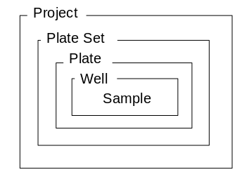
A project contains plate sets, each of which contains plates etc.
Projects can only be created by an administrator. Plate Sets can be
created by users. Other entities are created automatically as needed.
Plates, wells, samples are created at the time of plate set
creation.
Plates and wells are created automatically during rearraying
operations.
| Wallet ID: | ||
| License key: |
Once the license key is available, navigate to Utilities/Register menu item in the software and enter customer ID, license key and your email. These will be registered in a local database. This is a one time process.
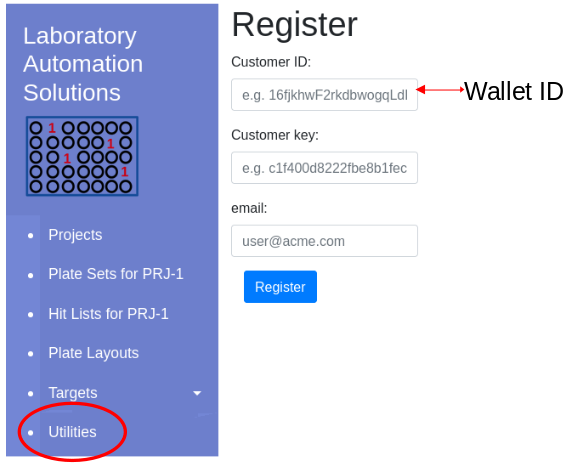
Click ‘Register’ to update the local database and confirm validity of the license key.
Problems?: info@labsolns.com Note that internet access is required for the licensing mechanism to work. If Blockchain.info is down, please try again at a later time.
Configuration of LIMS*Nucleus is achieved by editing either /etc/artanis/artanis.conf or $HOME/.config/limsn/artanis.conf, depending on how LIMS*Nucleus was installed. LIMS*Nucleus specific parameters are listed below:
These parameter will need to be edited if you utilize a cloud provider. These are the parameters that comprise the connection string. PostgreSQL is the only database with which LIMS*Nucleus is compatible.
| Parameter | Description | Default |
|---|---|---|
| db.addr | database address:port | 127.0.0.1:5432 |
| db.username | database username | ln_admin |
| db.passwd | database password | welcome |
| db.name | database name | lndb |
| Parameter | Description | Default |
|---|---|---|
| host.addr | Host address - the web server | 127.0.0.1 |
| host.port | web server port | 3000 |
| Parameter | Description | Default |
|---|---|---|
| cookie.expires | Cookie expiration time in seconds; Expiration of the session cookie will require a user to re-login | 21600 |
| cookie.maxplates* | Maximum number of plates per plate set; Modifications ignored unless registered | 10 |
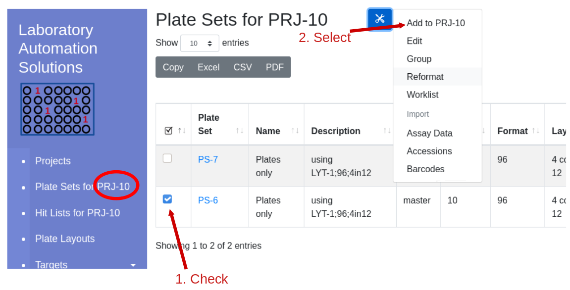
Click the ‘Projects’ hyperlink on the global navigation pane. Navigate into the project that will contain the plate set. Note that the ‘Plate Set For…’ link now indicates the default working project.
Select the check box near the plate set into which you would like to add a new plate set. Click the tools icon and select add to project…
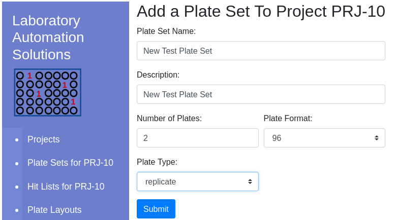
| Item | Notes |
|---|---|
| Type | Choose a descriptive type that can later be used for sorting |
| Layout | Check the Layout viewer to learn about the different layout options |
Available layouts are presented in the dropdown appropriate to the plate format/type:
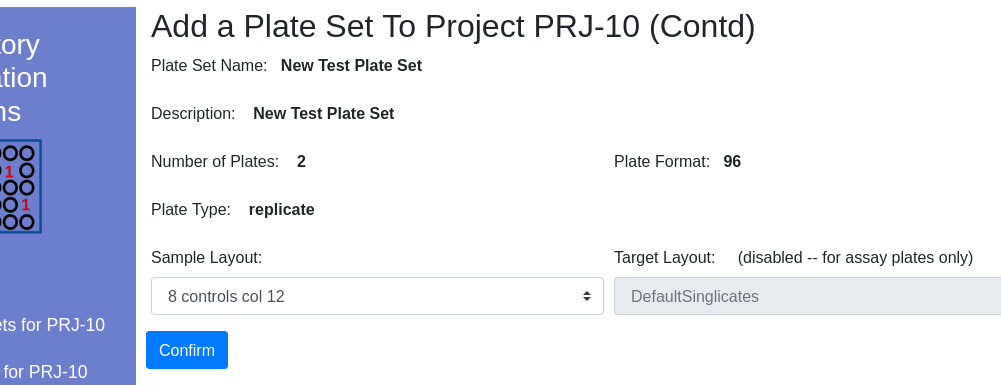
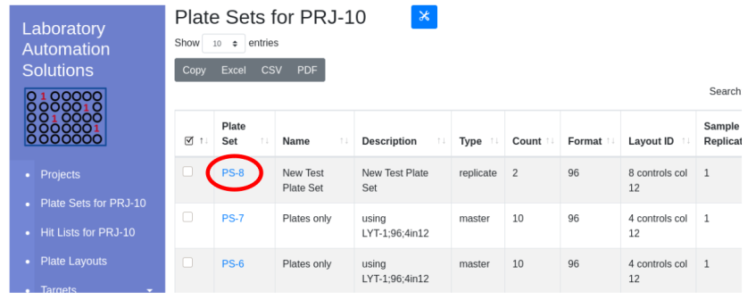
Once complete, the new plate set will be visible in the client window.
Email already exists.
Wallet/Customer ID not
generated.
Contact info@labsolns.com for assistance.
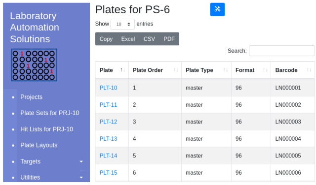
Barcode IDs are imported by plate number. The files page provides details on the file format, with a 10 plate sample file available. Navigate into the project of interest and highlight the plate set of interest. From the menu select Utilities/Import Barcodes:
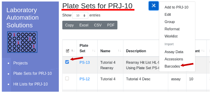
The import barcode form will appear - select file. A truncated sample of file contents will appear belwo the ‘Submit’ button for confirmation:
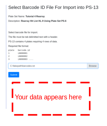
The example barcode import file looks like:
1 | plate barcode.id |
Once imported, barcode ids will appear in the plate table:
Example barcode ID import file:
| File name | Description |
|---|---|
| barcodes.txt | Ten 96 well plates in PRJ-10 |
| barcodes1000.txt | 1000 barcodes |
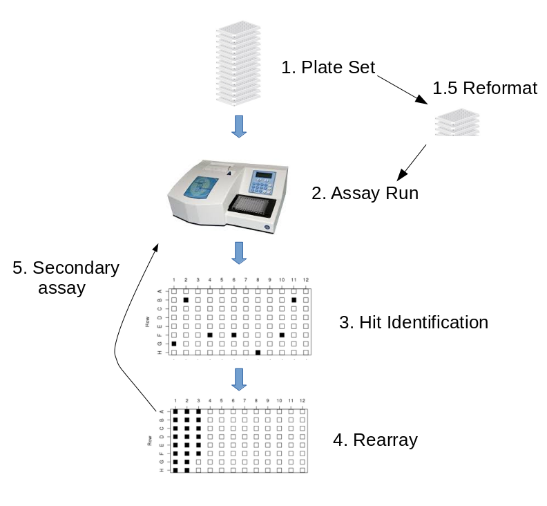
Below is the canonical workflow that LIMS*Nucleus is designed to handle.
Tutorial 1 will walk you through this workflow.
Thank you for your request.
An invoice in the amount of $5000 for a LIMS*Nucleus license key will be emailed to: