Plate

Plates are one of three formats - 96, 384, or 1536 well The plate system name in the format PLT-NNN is automatically assigned at creation All plates are part of plate sets

Plates can be assigned a variety of types. Depending on the type, a plate may not contain samples. For example, assay plates are transient and discarded after data collection, so could not serve as the source for rearraying or replica plating.

Installed types are:

Type Description Contain samples?
assay contain associated data no
rearray created during a reformat operation yes
archive designated for storage yes
master original plate of samples yes
daughter result of replica plating or grouping operations yes
replicate result of replica plating yes

Plates are of various types - assay, rearray, glycerol, etc. Plate types are to provide clarity to the user - no convention is enforced

PlateSet

Composed of plates Specific to a project All plates within a plate set must be of the same format (e.g. 96 well) Plate sets can be merged together (different plate types OK) When created, all plates in a plate set will be of the same plate type

PostgreSQL

View a schematic of the LIMS*Nucleus architecture here. If you have experience with PostgreSQL, you may wish to install the LIMS*Nucleus database independent of the client utilizing resources you already control e.g. an AWS instance of Postgres or Postgres running in your internal datacenter. This archive provides the necessary scripts for database installation/configuration. LIMS*Nucleus is agnostic with respect to the location of the database - all that is needed is a valid connection string. Once the database has been configured, the artanis configuration file must be modified.

Scripts included are:

Name Description
initdba.sql create users
initdbb.sql create database
initdbc.sql create schema and grant privileges to users
create-db-sql create tables, load functions, load required data e.g. layouts, plate types, assay types, etc.
example-data.sql load example data projects 1-10. Note this is not optional as LIMS*Nucleus will not boot without Project 1 in the database
drop-func-tables.sql used to refresh the database i.e. delete all user created data and reload required and example data
install-pg.sh install script that calls above scripts; see below for options

Once the database is up and running, install the client.

Postgres Install script

The postgres install script can be used to install a data directory under the current user, \(HOME/lndata, or to modify the database installed by <code>sudo apt-get install postgres</code> in the default data directory at /etc/postgresql/\)PGMAJOR/main

User directory

install-pg.sh
1
2
3
4
5
6
7
8
9
10
11
12
13
14
15
16
17
18
19
20
21
#!/bin/sh

mkdir lndata

echo "export PGDATA=\"$HOME/lndata\"" >> $HOME/.bashrc
export PGDATA="$HOME/lndata"
export LC_ALL="C"

sudo mkdir -p /var/run/postgresql
sudo chown -R admin:admin /var/run/postgresql
initdb -D $HOME/lndata

sed -i 's/\#listen_addresses =/listen_addresses =/' $HOME/lndata/postgresql.conf

pg_ctl -D $HOME/lndata -l logfile start

psql -U postgres -h 127.0.0.1 postgres -a -f initdba.sql
psql -U ln_admin -h 127.0.0.1 postgres -a -f initdbb.sql
psql -U ln_admin -h 127.0.0.1 -d lndb -a -f initdbc.sql
psql -U ln_admin -h 127.0.0.1 -d lndb -a -f create-db.sql
psql -U ln_admin -h 127.0.0.1 -d lndb -a -f example-data.sql

Take ownership with sudo chown -R admin:admin /var/run/postgresql where admin:admin is the user id

Default postgres directory

install-pg.sh
1
2
3
4
5
6
7
8
9
10
11
12
13
14
15
PGMAJOR=$(eval "ls /etc/postgresql")
PGHBACONF="/etc/postgresql/$PGMAJOR/main/pg_hba.conf"
sudo sed -i 's/host[ ]*all[ ]*all[ ]*127.0.0.1\/32[ ]*md5/host all all 127.0.0.1\/32 trust/' $PGHBACONF

PGCONF="/etc/postgresql/$PGMAJOR/main/postgresql.conf"
sudo sed -i 's/\#listen_addresses =/listen_addresses =/' $PGCONF

eval "sudo pg_ctlcluster $PGMAJOR main restart"

psql -U postgres -h 127.0.0.1 postgres -a -f initdba.sql
psql -U ln_admin -h 127.0.0.1 postgres -a -f initdbb.sql
psql -U ln_admin -h 127.0.0.1 -d lndb -a -f initdbc.sql
psql -U ln_admin -h 127.0.0.1 -d lndb -a -f create-db.sql
psql -U ln_admin -h 127.0.0.1 -d lndb -a -f example-data.sql

Create a Project

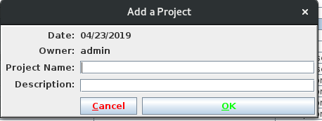
Only administrators can create/edit/delete projects. Project is the only entity that can be deleted. It will be deleted using a cascading delete, removing all plate sets, plates, samples, assay runs, and data that are part of the project. Access the “Add Project” menu item under the Admin menu - visible only to administrators:

A dialog will appear with 2 fields, name and description. Pressing OK will add to and refresh the project list in the main browser.

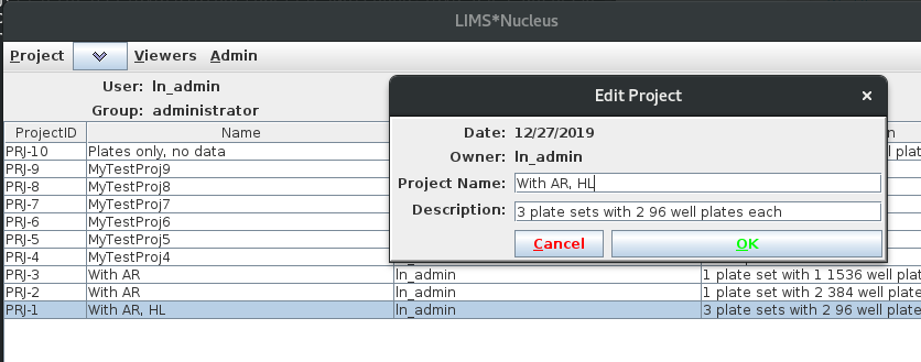
Edit Project

Select the project to be edited, then from the menu bar select Admin/project/edit. The edit project dialog box will be pre-populated with the selected project name and description. Make changes and save.

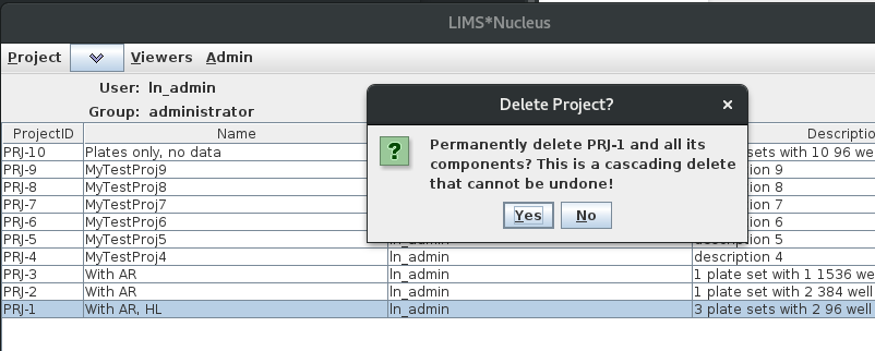
Delete Project

Select the project to be deleted and from the menu bar select Admin/project/delete. The delet project dialog box will be presented for confirmation,

Monoliths

LIMS (Laboratory Management Information Systems) can be broadly characterized into 2 groups, monoliths and systems. The difference is less about functionality and more about architecture. Monoliths are a large all inclusive application that maximize automation and minimizes user intervention. Monoliths are very efficient when a process is standardized and unchanging.

Advantages

  • Full automation, maximum reduction in FTE requirements
  • Consistant reproducible processing
  • Enhancements, upgrades, and training outsourced to the vendor
  • User groups provide resources for problem solving (bug fixes, add on components, help with problems)

Disadvantages

  • Cost
  • Many moving parts (database, ORM, web server, interface)
  • Complex - requires extensive training
  • Feature creep
  • Brittle - difficult to change in response to a changing process
  • Dependant on vendor for bug fixes and upgrades
  • Off-the-shelf solutions may not satisfy all requirements
  • May depend on obscure components (old programming languages, object database, image)
  • Custom solutions may be obsolete on delivery
  • Resistance to use

Next>> Systems

Mutation Visualization

Compare parental and mutant sequences

After perfoming error prone PCR (random) or oligonucleotide (directed) mutagenesis you will want to visualize your sequences and determine the rate of mutation incorporation. A typical visualization is the stacked bar chart as in this figure from Finlay et al. JMB (2009) 388, 541-558:
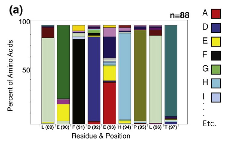
To decode this graphic you must:

  • estimate the percentage of each amino acid by comparison to the Y axis
  • compare relative amino acid abundance by comparing the area of boxes
  • correlate color with amino acid identity
  • compare to the reference sequence at the bottom of the graph

An easier to interpret graphic would be a scatter plot of sequence index (i.e. nucleotide position) on the X axis vs frequency on the Y. The data points are the single letter amino acid code. Highlight the reference sequence with a red letter.

The first step is to align all sequences. Start with a multi-fasta file of all sequences:


$cat ./myseqs.fasta

>ref
GLVQXGGSXRLSCAASGFTFSSYAMSWVRQAPGKGLEWVSAISGSGGSTYY
ADSVKGRFTISRDNSKNTLYLQMNSLRAEDTAVYYCAKDHRRPKGAFDIWGQGTMVTVSS
GGGGSGGGGSGGGGSGQSALTQPASVSGSPGQSITISCTGTSSDVGAYNYVSWYQQYPGK
APKLMIYEVTNRPSGVSDRFSGSKSGNTASLTISGLQTGDEADYYCGTWDSSLSAVV
>BSA130618a-A01
glvxxggxxrlscasgftfssyamswvrqapgklewvsaisgsggstyysdsvkgrftissdnskntlylqmnslraedt
avyycakdhrrpkgafdiwgqgtmvtvssggggsggggsggggsgqsaltqprsvsgtpgqsviisctgtssdvggskyv
swyqqhpgnapkliiydvserpsgvsnrfsgsksgtsaslaitglqaedeadyycqsydsslvvf
>BSA130618a-A02
glvqpggxxrlscasgftfssyamswvrqapgkglewvsaisgsggstyyadsvkgrftisrdnskntlylqmnslraed
tavyycakdhrrpngafdiwgqgtmvtvssggggsggggsggggsgqsvvtqppsmsaapgqkvtiscsgsssnignnyv
swyqqlpgtapklliydnnkrpsxipdrfsgsksgtsatlitglqtgdeadyycgtwdsslsagvf
>BSA130618a-A03
glvqxggxxrlscasgftfssyamswvrqapgkglewvsaisgsggstyyadsvkgrftisrdnskntlylqmnslraed
tavyycakdhrrpkgafdiwgqgtmvtvssggggsggggsggggsgsyeltqppsvsvspgqtasitcsgsssniginyv
swyqqvpgtapklliyddtnrpsgisdrfsgsksgtsatlgitglqtgdeadyycgtwdsslsvvvf

Above I have labeled my parental reference sequence “ref”. Use clustalo to perform the alignment and request the output in “clustal” format. The clustalo command can be run from within R using the system command. Read the alignment file into a matrix:

  input.file <- paste( getwd(), "/out.fasta", sep="")
  output.file <-  paste( getwd(), "/out.aln", sep="")
  system( paste("c:/progra~1/clustalo/clustalo.exe -infile=", input.file, " -o ", output.file, ".aln --outfmt=clustal", sep=""))   
 
 in.file <- paste(getwd(), "/out.aln", sep="")  
 seqs.aln <- as.matrix(read.alignment(file = in.file, format="clustal"))

At each position determine the frequency of all 20 amino acids. Set up a second matrix that has one dimension as the length of the sequence and the other as 20 for each amino acid. This is the matrix that will hold the amino acid frequencies.

The R package “seqinr” provides a constant containing all single character amino acids as well as asterisk for the stop codon. Use this to name the rows of the frequency matrix.

    library(seqinr)
levels(SEQINR.UTIL$CODON.AA$L)

[1] "*" "A" "C" "D" "E" "F" "G" "H" "I" "K" "L" "M" "N" "P" "Q" "R" "S" "T" "V"
[20] "W" "Y"

aas <- c(levels(SEQINR.UTIL$CODON.AA$L), 'X')
freqs <- matrix(  ncol=dim(seqs.aln)[2], nrow=length(aas))
rownames(freqs) <- aas

#Process through the matrix, calculating the frequency for each amino acid.
for( col in 1:dim(aligns)[2]){
     for( row in 1:length(aas)){
          freqs[row, col] <- length(which(toupper(seqs.aln[,col])==aas[row]))/dim(seqs.aln)[1]
      }
}

Set up an empty plot for Frequency (Y axis) vs nucleotide index (X axis). Y range is 0 to 1, X range is one to the length of the sequence i.e. the number of columns in the frequency matrix. Plot frequencies >0 in black, using the single letter amino acid code as the plot character.

    plot(1, type="n", xlab="Sequence Index", ylab="Frequency", xlim=c(1, dim(freqs)[2]), ylim=c(0, 1))
for( i in 1:length(aas)){
       points( which(freqs[i,]>0), freqs[i, freqs[i,]>0], pch=rownames(freqs)[i], cex=0.5)
       }

Overlay the reference sequence in red.

ref <-seqs.aln[rownames(seqs.aln)=="ref",]
for(i in 1:length(ref)){
     if(  length( freqs[rownames(freqs)[rownames(freqs)==toupper(ref[i])],i] ) > 0){
    if(freqs[rownames(freqs)[rownames(freqs)==toupper(ref[i])],i] > 0){
                  points( i,freqs[rownames(freqs)[rownames(freqs)==toupper(ref[i])],i]  , pch=toupper(ref[i]), cex=0.5, col="red")
              }
            }
    }

This is what it looks like (open in a new tab to see detail):

It’s easy to see which amino acid is parental, and its relative abundance to other amino acids is clear.
Consider position 61: N is the parental amino acid but T is now more abundant in the panel of mutants. K and S are the next most abundant amino acids.

Should multiple amino acids have the same or close to the same frequency, the graph can get cluttered and difficult to interpret. Adjusting the Y axis can help clarify amino acid identity. At each position percentages may not add up to 100 depending on the number of gaps. Consider the sequence “RFSGS” at positions 69-73 which is in a region containing gaps for some of the clones:

Installation

Edit your channels.scm file to include the labsolns channel

Once edited:


$guix pull
$guix package -i mutvis
$source $HOME/.guix-profile/etc/profile

##run the bash script

$mutvis.sh

General navigation

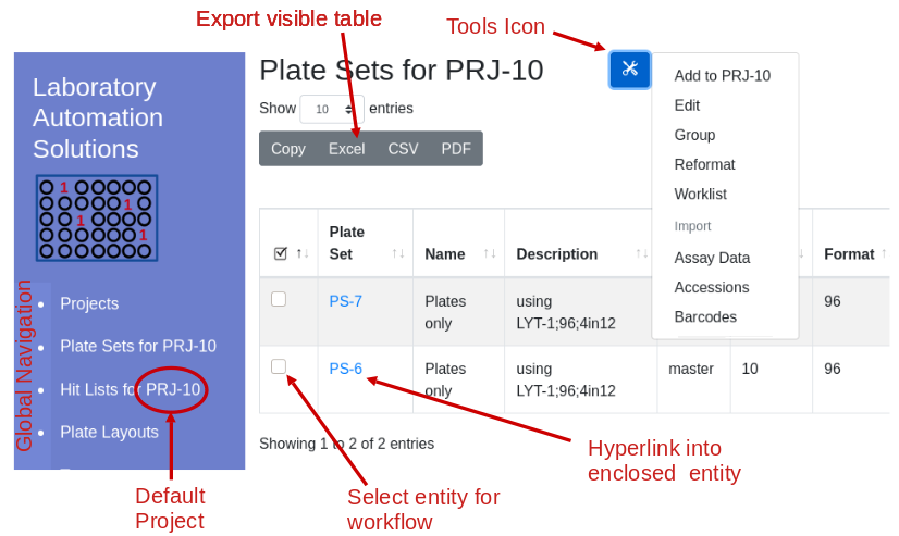
LIMS*Nucleus works with a nested heirarchy of entities. The object heirarchy can be navigted by clicking hyperlinks in the data tables. The left hand menu items allow for global navigation. Since users are often concerned with only one project at a time, LIMS*Nucleus tracks the current (default) project, which is visbile in the menu area. The default project can be changed by listing all project (first menu item) and clicking into a project. The tools icon presents workflows associated with the visible entity, and often require selection of row(s) in the data table.

hitlist

A list of samples of interest Must have a header road named “name” One sample per line, no separator Primarily used to cherry pick samples from plate to plate

Next:

Import Assay Data

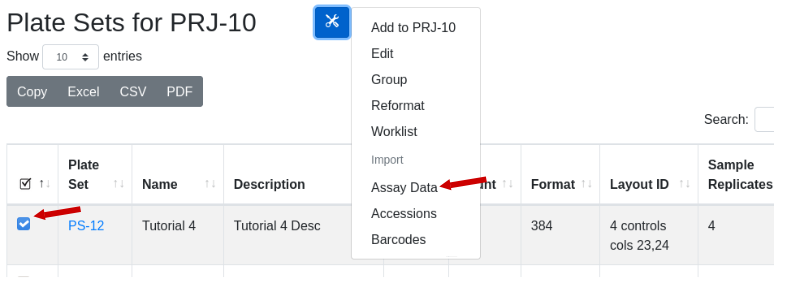
  1. Select the plate set that will receive the data

  2. From the tools icon under import select “Assay Data”

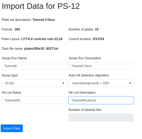
  1. A file import form will appear. Select the import file and submit. Fill in required data, making sure that the imported layout matches the defined layout of the plate set. Hit identification can be performed during import or deferred to a later time.

Once imported, the data can be viewed using a scatter plot, which is visible when viewing assay runs, i.e. click on the assay run hyperlink.

Layouts

LIMS*Nucleus makes use of the following definitions:

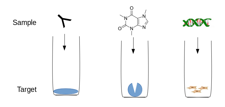
Sample: Item of interest being tracked by LIMS*Nucleus, i.e. the item in wells. Examples would be compounds, antibodies, bacterial clones, DNA fragments, siRNAs.

Target: the item with which the sample interacts, usually coated on the bottomn of the microwell plate e.g. the antigen for an antibody or the enzyme (target) of a compound.

When creating layouts there are three attributes that need to be defined:

Entity Attribute
Sample type, replication
Target replication

LIMS*Nucleus support 5 sample types:

Type ID
unknown 1
positive control 2
negative control 3
blank 4
edge 5

LIMS*Nucleus has twenty pre-defined layouts installed at the time of system installation. Custom sample layouts can be defined and imported by administrators. A sample layout import file that defines four control wells at the bottom of column 7 looks like:

1
2
3
4
5
6
7
8
9
10
11
12
13
14
15
16
17
18
19
20
21
22
well	type
1 1
2 1
3 1
4 1
5 1
...
51 1
52 1
53 2
54 2
55 3
56 4
57 1
58 1
...

92 1
93 1
94 1
95 1
96 1

When viewed in the layout viewer, the above file would provide the following sample layout:

For every sample layout imported, an additional 5 layouts are created that define sample and target replication. These layouts are discussed in detail on the replication page.

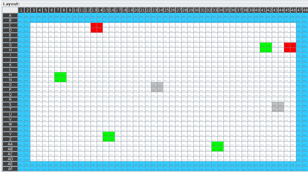
Here is a sample layout import file that defines 8 controls in a 384 well plate, randomly scattered, excluding edge wells

When reformatted into 1536, the layout will look like: